Project 6 - Extended kalman filter
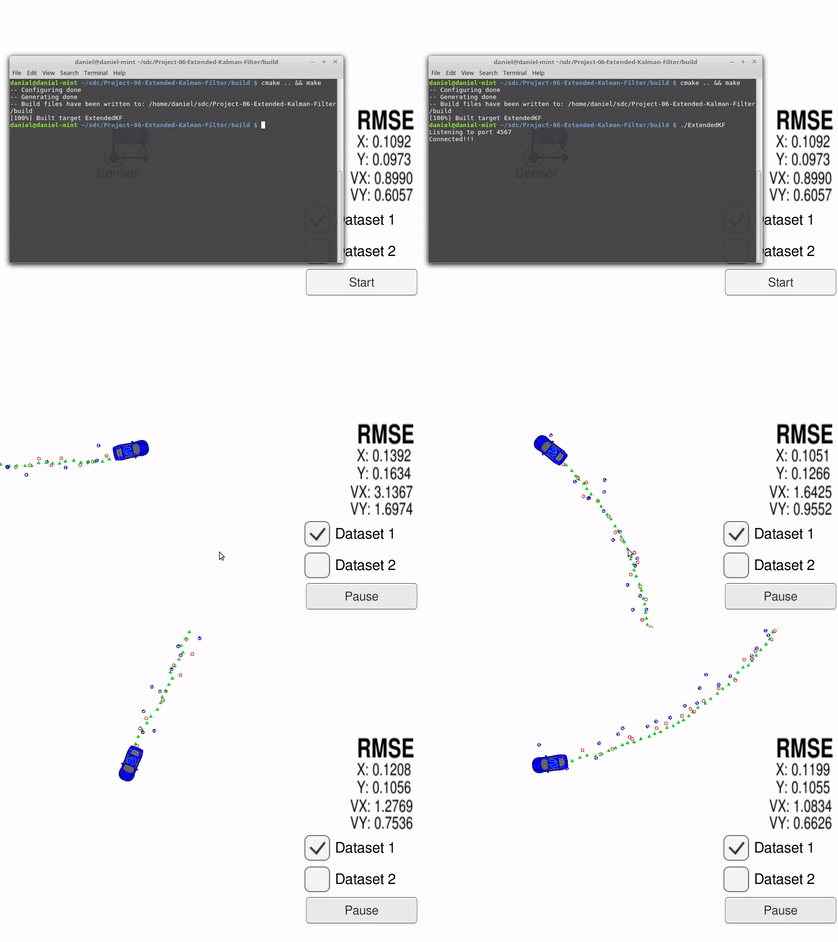
Red is Lidar measurements and blue is radar measurements. Green is the estimated location and heading produced by the Kalman filter. The car is the ground truth and as seen, green tracks it very accurately.
Filters are generally used to reduce the amount of noise in a signal so that useful information can be gathered about whatever you are trying to measure. One of the most basic filters is a moving average filter and it reduces the noise of a signal by taking an average of the previous n measurements.
For example, imagine you have a GPS device which has some noise when determining your location. GPS operate in multiple dimensions but let's pretend that the GPS is just trying to guess your position on a line that goes from 0 to 100 meters. If you're standing at the 10 meter location, 3 GPS measurements will read out something like 10.2 m, 10.1 m, 9.6 m. A moving average filter would then take the average of these three values and yield 9.97 m, an estimate very close to your exact location. One obvious draw back of a moving average filter is the time delay, but if your standing still thats okay.
However what will happen if, like the car shown on the left, you are in motion. Imagine you write down the GPS measurement and then move 5 meters. Using a moving average filter to guess your new location will be more than 5 meters behind! Let's simulate three movements. You write down the GPS reading 9.6 m and move to location 15 m. You write down 15.2 m and move to 20 m. You write down 19.9 m and move to 25 m. Where does your moving average filter think you are? (9.6 + 15.2 + 19.9)/3 = 14.9 m, but really you are at the 25 m location.
A Kalman filter uses a state transition function and then tries to determine the coefficients of this function. In the example above, we are moving with a set velocity and ending up at a new location every time step. Thus the state transition function we would program into the Kalman filter would be: prev_loc + vel = new_loc. Then using the information we measure, the Kalman filter would try to estimate our velocity. For the three time steps we measured, it could estimate the velocity twice. vel = 15.2 - 9.6 = 5.6, and vel = 19.9 - 15.2 = 4.7. Let's assume the Kalman filter estimates the velocity to be 5.15 after these two measurements (this wouldn't be exactly true in practice).
With an accurate estimate of the velocity, the Kalman filter could then better predict the next location. When we write down a GPS reading of 19.9 m and move to location of 25 m, the Kalman filter would predict our new location to be 25.05 m. Much closer than the estimate given by the moving average filter! It would use the state transition function above, put in 19.9 in prev_loc, and 5.15 in vel and add them together to get new_loc. I hope with this simple example you ca see how a Kalman filter succeeds where a more basic filter fails.
In this project, we have a stationary set of sensors that is trying to track the blue car as shown in the gif. A basic moving average filter would be unable to accurately predict the targets next location as shown by the previous example. Another reason the Kalman filter is perfect for this problem is that it can use multiple different sensors. LiDAR measurements give you an objects X,Y position relative to your position. A radar sensor will give you the objects angle, distance, and velocity. When using a Kalman filter, it is fairly easy to combine these measurements and use them in determining the coefficients of a single state transition matrix. Then this common state transition matrix can be used to make predictions about the targets new location.
Project 7 - unscented kalman filter
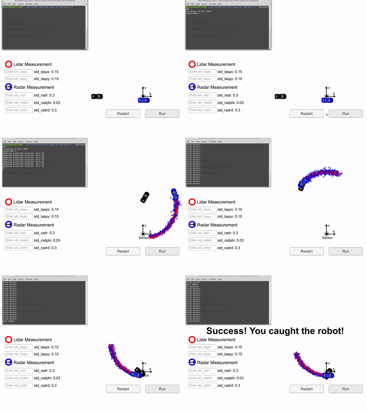
The hunter car (black) is uses an Unscented Kalman filter to predict where the blue car will be to catch it.
An Unscented Kalman filter (UKF) performs better than an EKF when the faced with non-linear process models or non-linear measurement models. The UKF uses a sampling technique to more accurately represent any non-lineararties present in the covariance. A more accurate covariance will yield a better estimate of the true state.
The gif to the left shows the UKF in action. Both the hunter car (black) and the target car (blue) have the same max velocity. Thus the hunter car has to use the UKF's prediction of where the blue car will be in the future in order to catch it.
The algorithm I used to catch the blue car had 3 modes. First the black car uses a prediction relative to the distance between it and the blue car to close the distance. Once within a set distance, the black car will drive to where the blue car will be 2 seconds from now. Once it gets to this point it will then turn around and drive directly at the blue car in order to meet it head-on.
In the gif you can see that the first time the black car drives directly at the blue car, it misses. This is because the black car doesn't know the blue cars exact position, it has to use the UKF to predict where it will be. It then follows the blue car for a bit before again predicting where it will be 2 seconds from now and driving there. The second time it drives straight at the blue car, it manages to catch it.
Project 8 - Particle Filter
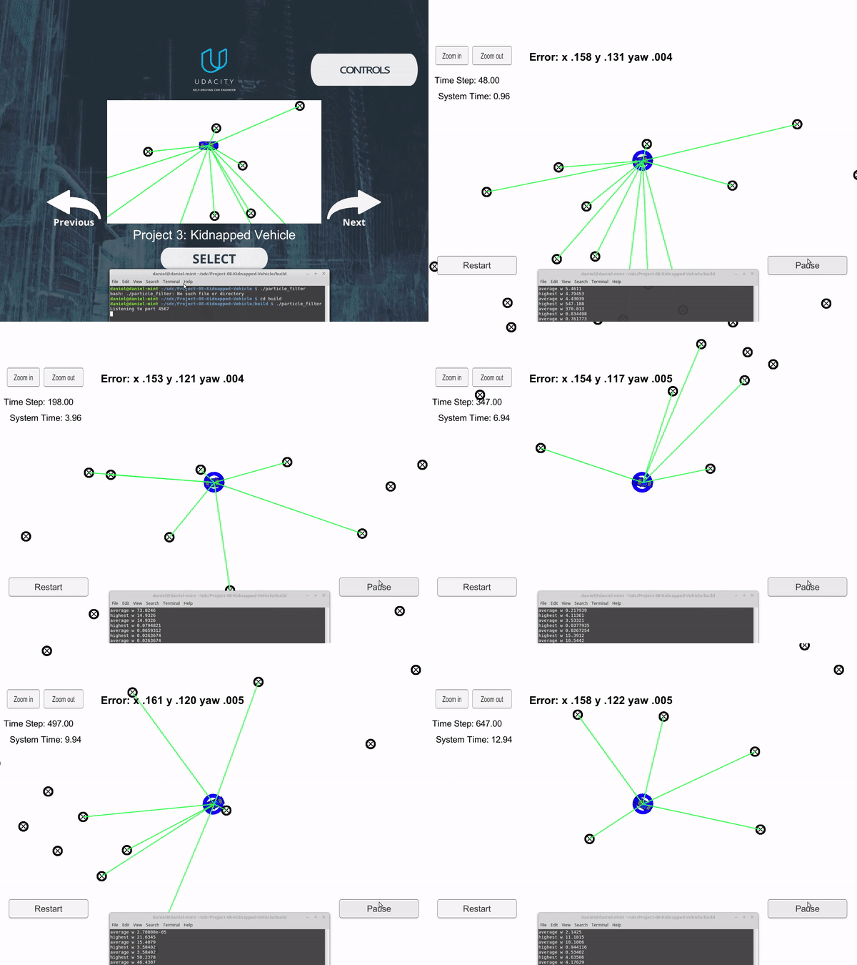
Blue circle is the particle filter guess, and the blue car is the true car position.
A particle filter is a probabilistic algorithm that is very well suited for localization. As shown on the left, the blue circle is trying to guess where the blue car is located. This is a localization problem. The only measurement inputs are the distance and angle of all objects within a specific radius. These measurements are shown by the green lines. The particle filter also has a global map which contains the location of all the objects. However, it doesn't know that a specific measurement corresponds to a specific object. In other words it doesn't know when it measures an object, where that object is on the global map.
To solve this localization problem, the particle filter first populates the global map with tens or hundreds of cars placed at random locations facing random directions. Then it will compare it's current measurements (of an objects distance and angle to it) to each of the randomly generate cars. Since it has placed these cars on the global map, the algorithm knows the distance of all objects and their angle to the car. This can then be compared to the real measurements to see how well they fit. If the car measures one object at 90 degrees and 1 m away and a randomly generated car measures 5 objects, the fit will be poor. However if another random car measures one object at an angle of 70 degrees and 0.9 m away, the fit will be good.
Once it has gone through all the randomly generated cars and determined their fit to the real measurements, the next batch of randomly generated cars will have a higher probability of being placed close to and in the same heading as the cars with the best fit. This process will continue constantly. For the gif, the blue circle is the particle that has the highest fit with the real measurements for that time step.
project 9 - PID control
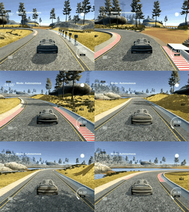
PID is wobbly because it is a purely reactive controller. It doesn't predict ahead.
A PID controller is one of the most widely used control systems and should almost always be the first tool attempted on a new control problem. In this project we attempted to use a PID controller to steer the car around the track. The car is continuously given it's distance from the center of the lane. In a real self driving car this could be provided by one of the localization techniques we learned previously in this term.
While a PID controller can navigate the car around the track, as shown in the gif, it's far from optimal. The main reason for this is that a PID controller is a purely reactive controller. If a sharp turn is coming up, it won't do anything about it until it starts moving away from the center line of the road.
A PID reacts (by turning the steering wheel) only to the error supplied to it (which in this case is the distance from the cars current location to the center line of the road). P, I, and D stand for proportional, integral, and derivative, which are the 3 ways the controller reacts to the error. These 3 portions of the controller are then summed together to produce the controllers output (steering the car).
If the error is large, the controller output (steering) will be large. If the error is small, the controller output will be small. This is the proportional part of the controller. The same goes for the direction of steering. An integral at it's most basic level is a sum. If there is a small but consistent error, the integral term will start small and eventually grow larger until that error is reduced. Imagine if the cars steering had some small offset. The integral portion of the controller would accumulate (sum) this build up of resulting error and eventually counter it. A derivative corresponds to change. Thus the derivative portion of the controller measures the change in error and reacts to it. If the change in error is large, the derivative portion of the controller is large.
For a car driving along a track, the derivative portion of the controller is extremely important. Imagine the PID has the controller steering hard toward the centreline. However, ideally the car shouldn't approach the centreline at a sharp angle or with a high rate of speed as it's going to overshoot the center and keep going. In this case the change in error would be large, but it would be a large reduction in error (because the car is rapidly closing in on the center line). Thus the derivative portion of the controller is used to slow down this rapid reduction in error so the car will approach the center line more smoothly.
Project 10 - Model predictive control
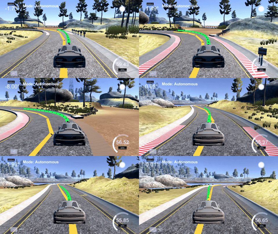
The yellow line is the path the car wishes to follow (which has localization error) and the green path is the one generated by the MPC as the route the car will take.
A model predictive controller (MPC) is a control system that use dynamics models to optimize the system response over a number of time steps. Unlike the PID controller, the MPC doesn't just react, but also predicts and optimizes based on those predictions.
For this project we had to determine the dynamic model and the cost function used by the controller. The cost function is equivalent to the error of a PID. You load up a cost function with the things you want to avoid. For this project part of the cost function was the distance between the car and the center of the road. However other costs can be used as well to get a more optimal solution. Some other parts of the cost function included the change in steering input (rapidly changing steering inputs lead to jerky ride and should be avoided), the cars acceleration, and the difference in angle between the cars heading and the center line heading.
MPC works by optimizing it's control outputs (steering) to achieve a minimum cost. In other words, the controller will use the dynamic model to predict how a set of control outputs will change the cars state and thus affect the cost function. While the controller produces a set of control outputs for all the time steps of its prediction horizon (shown in green), it only executes the first control output before starting the process all over again for the next time step.
All the code for these projects can be found on my GitHub page.

